3D MHD Test: Magnetosphere

地球磁気圏に太陽風が吹き付け、地球磁気圏が変形する様子をシミュレーションします。[Ogino, 1986]を参考にして、地球の中心から地球半径の3.5倍の位置にも境界を設置し、地球の双極子磁場とスムーズに接続するようにしています。

Location

demo/mhd3d_magnetosphere/

Normalization

物理量は以下の代表値で規格化しています。[Ogino, 1986]ではMKS単位系が使われていますが、本シミュレーションではcgs単位系を使用していることに注意してください。

Quantity	Symbol	Value	Note
Length	\(R_\mathrm{e}\)	\(6.371 \times 10^8~\rm{cm}\)	Earth radius
Magnetic Field	\(B_\mathrm{s}\)	\(3.12 \times 10^{-1}~\rm{G}\)	Strength at earth equator surface
Density	\(\rho_\mathrm{s}\)	\(1.67 \times 10^{-20}~\mathrm{g~cm^{-3}}\)	Typical density of ionosphere

Then the other quantities are normalized as follows.

Quantity	Symbol	Value
Velocity	\(V_\mathrm{s}\)	\(B_{\rm{s}}/\sqrt{4\pi \rho_{\rm{s}}}=6.81\times 10^8~\rm{cm~s^{-1}}\)
time	\(t_\mathrm{s}\)	\(R_{\rm{e}}/V_{\rm{s}}=0.935~\rm{s}\)
Pressure	\(p_\mathrm{s}\)	\(B_{\rm{s}}^2/4\pi=7.74\times 10^{-3}~\rm{dyn~cm^{-2}}\)

Geometry

• \(-44.8 \leq x \leq 44.8\)

• \(-44.8 \leq y \leq 44.8\)

• \(-44.8 \leq z \leq 44.8\)

Force

地球の中心に向かう重力を考慮します。

\[\begin{split} \begin{align*} \frac{\partial \rho \bm{v}}{\partial t} &= [...] + \rho \bm{g}, \\ \bm{g} & = -\frac{g_0}{r^3} \left(x \bm{e}_x + y\bm{e}_y + z\bm{e}_z\right),\\ r^2 &= x^2 + y^2 + z^2, \end{align*} \end{split}\]

where \(g_0=1.35\times10^{-6}\) in normalized unit.

Initial Conditions

初期条件は、磁気圏と太陽風の組み合わせで記述されます。比熱比は\(\gamma = 5/3\)とします。

密度

\[\begin{split} \begin{align*} \rho &= \begin{cases} 1/r^3 & 1/r^3 \geq 0.2\rho_\mathrm{sw} \\ 0.2\rho_\mathrm{sw} & 1/r^2 < 0.2\rho_\mathrm{sw} \end{cases} \end{align*} \end{split}\]

圧力

\[\begin{split} \begin{align*} p = \begin{cases} p_0/r^2 & p_0/r^2 \geq p_\mathrm{sw} \\ p_\mathrm{sw} & p_0/r^2 < p_\mathrm{sw} \end{cases} \end{align*} \end{split}\]

双極子磁場

\[\begin{split} \begin{align*} \bm{B} &= \frac{1}{r^5} \begin{pmatrix} -3xz \\ -3yz \\ x^2 + y^2 - 2z^2 \end{pmatrix} \end{align*} \end{split}\]

ここで\(p_0 = 5.4\times10^{-7}\)。 太陽風のパラメータは、\(\rho_\mathrm{sw}=5\times10^{-4}\)、\(p_\mathrm{sw}=3.56\times10^{-8}\)、\(v_\mathrm{sw}=0.05\)、\(B_\mathrm{sw}=-1.5\times10^{-4}\)です。

Boundary Conditions

すべての境界に対して、\(x = -44.8\)境界を除き、全ての物理量に対して対称境界条件を設定します。\(x = -44.8\)境界では、上記の太陽風のパラメータを固定境界条件として設定します。config.yamlでは以下のように設定します。加えて、地球周辺(\(r = 3.5R_\mathrm{E}\))に境界のような条件を設定し、双極子磁場とスムーズに接続するようにしています。

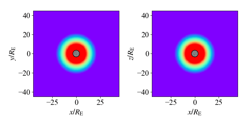
Results

可視化用のPythonスクリプトが用意されています。 結果のプロットは demo/mhd3d_magnetosphere/figs に保存されます。

cd demo/mhd3d_magnetosphere
python plot_data.py