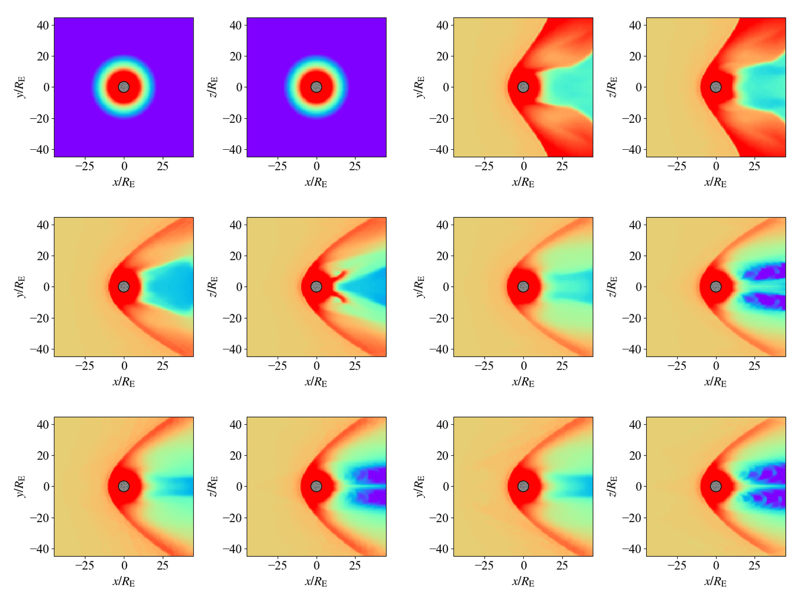
3D MHD Test: Magnetosphere

This simulates how the solar wind blows against Earth’s magnetosphere and deforms it. Following [Ogino, 1986], we also place a boundary at 3.5 Earth radii from the center of the Earth and connect it smoothly to the Earth’s dipole magnetic field.

Location

demo/mhd3d_magnetosphere/

Normalization

The variables are normalized by the following typical values. Note that [Ogino, 1986] uses MKS units, whereas this simulation uses cgs units.

Quantity	Symbol	Value	Note
Length	\(R_\mathrm{e}\)	\(6.371 \times 10^8~\rm{cm}\)	Earth radius
Magnetic Field	\(B_\mathrm{s}\)	\(3.12 \times 10^{-1}~\rm{G}\)	Strength at earth equator surface
Density	\(\rho_\mathrm{s}\)	\(1.67 \times 10^{-20}~\mathrm{g~cm^{-3}}\)	Typical density of ionosphere

Then the other quantities are normalized as follows.

Quantity	Symbol	Value
Velocity	\(V_\mathrm{s}\)	\(B_{\rm{s}}/\sqrt{4\pi \rho_{\rm{s}}}=6.81\times 10^8~\rm{cm~s^{-1}}\)
time	\(t_\mathrm{s}\)	\(R_{\rm{e}}/V_{\rm{s}}=0.935~\rm{s}\)
Pressure	\(p_\mathrm{s}\)	\(B_{\rm{s}}^2/4\pi=7.74\times 10^{-3}~\rm{dyn~cm^{-2}}\)

Geometry

• \(-44.8 \leq x \leq 44.8\)

• \(-44.8 \leq y \leq 44.8\)

• \(-44.8 \leq z \leq 44.8\)

Force

We take into account gravity directed toward the center of the Earth.

\[\begin{split} \begin{align*} \frac{\partial \rho \bm{v}}{\partial t} &= [...] + \rho \bm{g}, \\ \bm{g} & = -\frac{g_0}{r^3} \left(x \bm{e}_x + y\bm{e}_y + z\bm{e}_z\right),\\ r^2 &= x^2 + y^2 + z^2, \end{align*} \end{split}\]

where \(g_0=1.35\times10^{-6}\) in normalized unit.

Initial Conditions

The initial condition is described by a combination of the magnetosphere and the solar wind. The ratio of specific heats is \(\gamma = 5/3\).

Density

\[\begin{split} \begin{align*} \rho &= \begin{cases} 1/r^3 & 1/r^3 \geq 0.2\rho_\mathrm{sw} \\ 0.2\rho_\mathrm{sw} & 1/r^2 < 0.2\rho_\mathrm{sw} \end{cases} \end{align*} \end{split}\]

Pressure

\[\begin{split} \begin{align*} p = \begin{cases} p_0/r^2 & p_0/r^2 \geq p_\mathrm{sw} \\ p_\mathrm{sw} & p_0/r^2 < p_\mathrm{sw} \end{cases} \end{align*} \end{split}\]

Dipole magnetic field

\[\begin{split} \begin{align*} \bm{B} &= \frac{1}{r^5} \begin{pmatrix} -3xz \\ -3yz \\ x^2 + y^2 - 2z^2 \end{pmatrix} \end{align*} \end{split}\]

Here \(p_0 = 5.4\times10^{-7}\). The solar wind parameters are \(\rho_\mathrm{sw}=5\times10^{-4}\), \(p_\mathrm{sw}=3.56\times10^{-8}\), \(v_\mathrm{sw}=0.05\), and \(B_\mathrm{sw}=-1.5\times10^{-4}\).

Boundary Conditions

A symmetric boundary condition is imposed on all variables at all boundaries except the \(x = -44.8\) boundary. At the \(x = -44.8\) boundary, the solar wind parameters above are imposed as a fixed boundary condition. This is set in config.yaml as follows. In addition, a boundary-like condition is imposed around the Earth (\(r = 3.5R_\mathrm{E}\)) so that it connects smoothly to the dipole magnetic field.

Results

A Python script for visualization is provided. The plots of the results are saved in demo/mhd3d_magnetosphere/figs.

cd demo/mhd3d_magnetosphere
python plot_data.py